Prior articles in this series
- Introduction to GIS Analysis using Sasquatch Sightings
- Spatial Squatch – Using the ArcGIS Pro Spatial Statistics Toolbox to Identify Sighting Patterns
- Mapping Clusters of Sasquatch Sightings
- Sasquatch Sighting Heat Maps with R
In this article I’ll show you how easy it can be to create 3D maps in R using the rayshader package. rayshader is an open source package for producing 2D and 3D data visualizations in R. rayshader uses elevation data in a base R matrix and a combination of raytracing, spherical texture mapping, overlays, and ambient occlusion to generate beautiful topographic 2D and 3D maps. In addition to maps, rayshader also allows the user to translate ggplot2 objects into beautiful 3D data visualizations.
The models can be rotated and examined interactively or the camera movement can be scripted to create animations. Scenes can also be rendered using a high-quality pathtracer, rayrender.The user can also create a cinematic depth of field post-processing effect to direct the user’s focus to important regions in the figure. The 3D models can also be exported to a 3D-printable format with a built-in STL export function.
Before we get to the code let’s look at an example of the output from the script we’ll write. I often find that it makes understanding the code easier if you can see an example of what will be produced. Below is a video of the animated 3D map that we’ll produce, which displays the number of Sasquatch sightings by county and is color coded and extruded into three dimensions. Consistent with what we’ve seen in past articles we see high concentrations of sightings in the counties just south of Tacoma, WA near Mount Rainier south through the Cascade Mountains toward Mount St. Helens and down into north central Oregon. Smaller clusters are found on the Olympic Peninsula and north of Seattle.
Now let’s see how this map was produced with R using the tidyverse, rayshader, sf, and viridis packages. You can download the R script and shapefile used to produce this map. We could just as easily used a feature class from a file geodatabase as a shapefile. The sf (simple feature) package in R supports both.
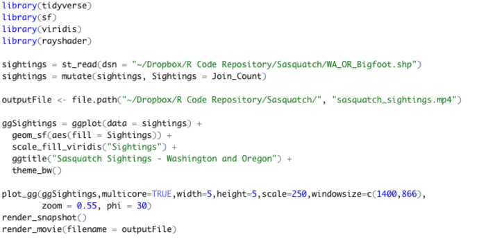
Here is the full script.
Loading the Packages
The first few lines of code simply load the R packages that will be used in the script including tidyverse, sf, rayshader, and viridis. I described the rayshader package above. The tidyverse package is actually a collection of packages for data loading, manipulation, tidying, exploration, and visualization for data science. Specific to this script, it also loads the ggplot2 package, which will be used to create the color coded map.
This script also uses the sf package to load the shapefile into an R data frame, which is basically a tabular structure that in this case also includes a column containing the spatial data (polygons in this case). The viridis package is used for to define the color coding for the map.
Loading and Preparing the Sighting Data
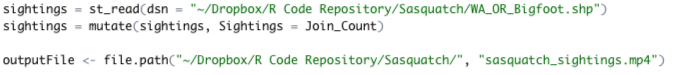
The next few lines of code load the shapefile into a data frame, rename the Join_Count field to Sightings, and define an output file location and name for the animation that will be created. This shapefile (WA_OR_Bigfoot.shp) contains a Join_Count field that was produced in ArcGIS Pro in a previous article using the Spatial Join geoprocessing tool. It simply contains the number of sightings per county. We’re just renaming this field to “Sightings” with the tidyvderse mutate() function.
Creating the Map
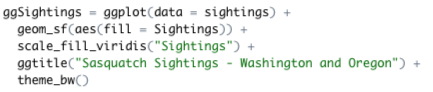
To produce the map, we use the ggplot() function from the ggplot2 package. The ggplot() function accepts a dataset, which is defined through the sightings data frame imported from the WA_OR_Bigfoot shapefile. The geom_sf() function loads the polygon data from the Sightings field, and we also define the color coding through scale_fill_viridis() function that accepts a column (Sightings) to define the color coding. Finally, we give our map a title and define the output theme.
Use rayshader to Plot Data in 3D
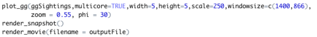
The final lines of this script use the plot_gg() function from the rayshader package to display the data in 3D. Notice that the ggSightings variable, produced by the ggplot() function is passed to the plot_gg() function. The render_snapshot() function creates the 3D rendering, and render_movie() creates the mp4 video.
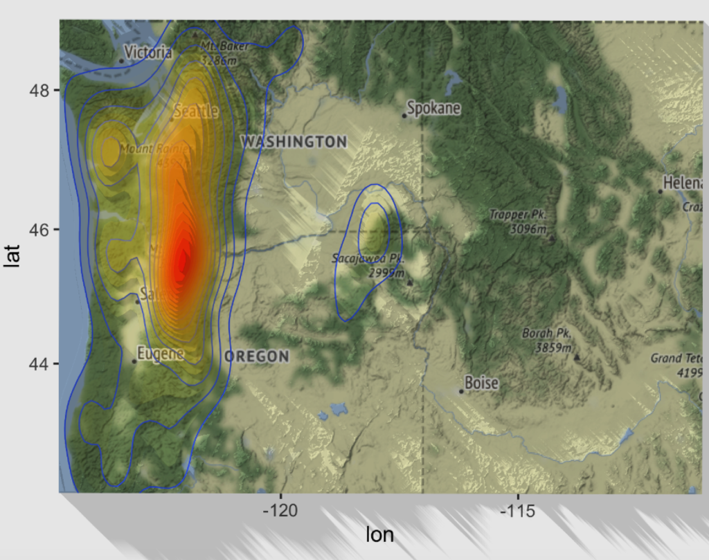
Another 3D Map of Sasquatch Sightings
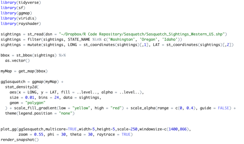
You can see an alternative 3D map of Sasquatch sightings that I produced from the point data below. The rayshader package was used to produce this map as well along with a Google Maps basemap produced with the ggmap package.
Here is the code used to produce this 3D map.