

In the first article in this series – Introduction to GIS Analysis using Sasquatch Sightings – you learned how to use basic ArcGIS Pro tools for spatial analysis. As with most other GIS projects there is always a significant amount of data preparation and processing, and that was the primary focus of the initial article. After downloading a dataset of Sasquatch sightings in North American we converted the data to a GIS format, created a subset of this dataset focused on the Pacific Northwest, and spatially joined the data to a feature class of counties. After that initial data preparation we then created some basic graduated color maps and examined summary statistics.
In this article we’ll take the spatial analysis one step further by using several tools from the Spatial Statistics Tools toolbox. Specifically, we’ll use several tools from the Measuring Geographic Distributions toolset. The Measuring Geographic Distributions toolset contains a set of tools that provide descriptive geographic statistics. Together, this toolset provides a set of basic statistical exploration tools. We will also learn how to use Average Nearest Neighbor tool to measure the presence or absence of clustering in a dataset.
Getting Started
We’ll pick up where we left off with the first article in this series so at this point you should already have an ArcGIS Pro Bigfoot project that you’ll need to open.
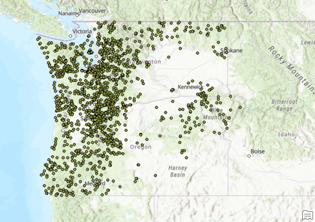
For today’s article we’ll focus specifically on the states of Washington and Oregon. Using your ArcGIS Pro skills create a new feature class called WA_OR_Bigfoot_Points that only contains sightings for Washington and Oregon. Hint: Use the Select by Location tool to facilitate this. The result should be as appears in the screenshot below.
Very Important!
Before we go any further I should point out that for most of the tools found in the Spatial Statistics toolbox you will need to use projected data. These tools require accurate distances and the WGS84 coordinate system so often used today for display purposes doesn’t measure distance accurately.
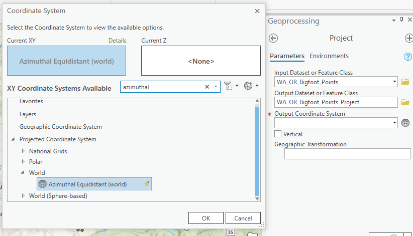
Use the Project tool in ArcGIS Pro to project WA_OR_Bigfoot_Points to create a new feature class called WA_OR_Bigfoot_Points_Project using a projected coordinate system of World | Azimuthal Equidistant which should minimize distance distortion.
Measuring Geographic Distributions
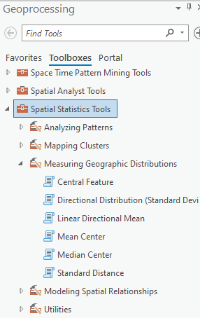
The Measuring Geographic Distributions toolset in the Measuring Geographic Distributions toolbox contains a set of tools that provide descriptive geographic statistics including the central feature, directional distribution, linear directional mean, mean center, median center, and standard distance. The are tools that provide basic descriptive spatial statistical information about a dataset.
In ArcGIS Pro go to the Analysis tab and click Tools to display the Geoprocessing pane (known as ArcToolbox in ArcGIS Desktop). Find the Spatial Statistics toolbox and then the Measuring Geographic Distributions toolset.
Central Feature
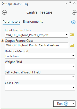
The Central Feature Tool identifies the most centrally located feature from a point, line, or polygon feature class. It adds and sums the distances from each feature to every other feature. The one with the shortest distance is the central feature. This tool creates an output feature class containing a single feature that represents the most centrally located feature. In our case, the tool will identify the Sasquatch sighting that is the central most location from the group.
Run the tool with the parameters specified below. Note that you could also run this tool with the BigFootByCountyPNW feature class using Join_Count as the Weight Field. In this case though since we’re just providing point feature class input there is no need to include a weight field.
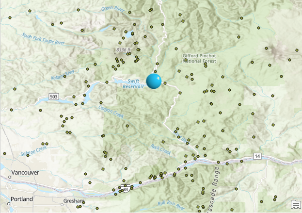
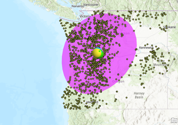
The Central Feature tool has identified the point as being just to the Northeast of the Portland, OR metro area and within the Gifford-Pinchot National Forest. This will come as no surprise to anyone who follows this topic closely. There have been many, many sightings in this area over the years.
Median and Mean Feature
The Mean Center tool calculates the geographic center for a set of features and can also be weighted by a numeric field. One thing to keep in mind when using this tool is that outliers can dramatically alter the mean. So, if your data contains outliers you might be better off using the Median Center tool which is also easier to calculate.
The Median Center tool identifies the location from a feature class that minimizes the overall Euclidean distance to the features in a dataset. Unlike the Mean Center Tool, the Median Center tool is not as affected by outliers.
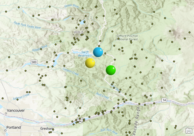
Run the Mean Center and Median Center tools to create the output you see below. It is not necessary to use any of the optional parameters including weight and case field for this exercise. Median center is displayed in yellow, mean center in green, and central feature in yellow. All display roughly the same sense of where is the center of my dataset.
Want to learn more about spatial analysis in ArcGIS Pro? Take a look at our Introduction to Spatial Analysis with ArcGIS Pro and R class.
Directional Distribution
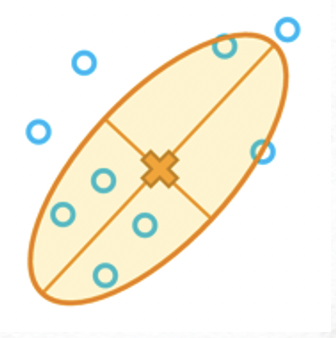
The Directional Distribution or Standard Deviational Ellipse tool creates standard deviation ellipses to summarize the spatial characteristics of geographic features including central tendency, dispersion, and directional trends. The ellipses are centered on the mean center. This tool calculates directionality, centrality, and dispersion. The image below depicts a typical output from this tool and displays the three characteristics of central tendency, dispersion, and directional trend. Here there is a pretty strong northeast to southwest directional trend, and a tight clustering of data indicated by a fairly narrow ellipse. A thicker ellipse would indicate a wider dispersal of data.
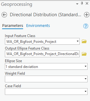
Run the Directional Distribution tool with the parameter below including 1 standard deviation and no weight or case field.
The output should appear as seen below. This basically looks like a blob but it does give us some important information through it’s elliptical shape. 68% of the sightings fall within this polygon boundary (1 standard deviation). This tool provides us with some sense of the directionality of the sightings and the dispersion. There appears to be some northeast to southwest directionality that roughly follows the Cascade Mountains of the two states. The thickness of the output polygon indicates a wide dispersal of sightings.
Average Nearest Neighbor
The Analyzing Patterns toolset in the Spatial Statistics Toolbox contains a series of tools that help evaluate if features or the values associated with features form a clustered, dispersed, or random spatial pattern. These tools generate a single result for the entire dataset in question. Tools in this category generate what is known as inferential statistics or the probability of how confident we are that the pattern is either dispersed or clustered.
These tools don’t produce a map! They simply give us an indication of whether or dataset shows a statistically significant clustering or dispersion of data or whether the data simply exhibits a random pattern.
Before we can move on to the hot spot and cluster analysis tools we need to first check our dataset to make sure the data is clustered or dispersed and not random. There are several tools that can be used to perform this type of test in the Analyzing Patterns toolset, but for this article we’ll just run the Average Nearest Neighbor tool.
The Average Nearest Neighbor tool calculates a nearest neighbor index based on the average distance from each feature to its nearest neighboring feature. For each feature in a dataset the distance to its nearest neighbor is computed. An average distance is then computed. The average distance is compared to the expected average distance. In doing so, an ANN ratio is created which in simple terms is the observed / expected. If the ratio is less than 1 we can say that the data exhibits a clustered patterns whereas a value greater than 1 indicates a dispersed pattern in our data.
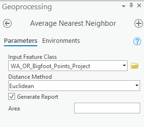
Find the Average Nearest Neighbor tool and open it. Provide the following input parameters (make sure you check Generate Report). Run the tool.
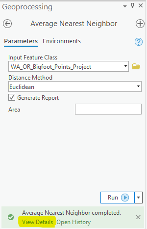
Open the output report file. You can find the location of the file by clicking View Details below the Run button and then clicking the link
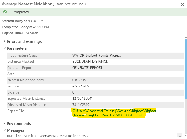
The output report should appear as seen below.
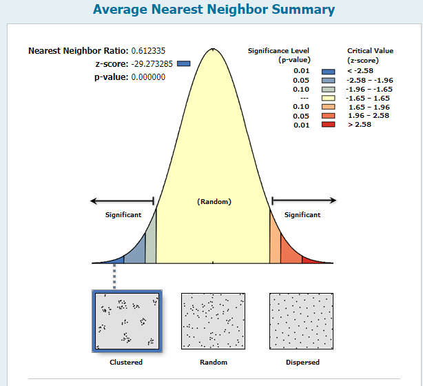
The ANN ratio created as a result of dividing the observed distance by the expected distance creates a value between 0 and 1. If the ratio is less than 1 we can say that the data exhibits a clustered patterns whereas a value greater than 1 indicates a dispersed pattern in our data.
The Sasquatch sightings data appears to have a clustered pattern. What we didn’t want was a random pattern. Clustered or dispersed is fine for purposes of moving on to the next series of tools involving hot spot analysis and cluster analysis.
In the next article in this series we’ll examine several tools for mapping clusters of Sasquatch sightings including Hot Spot Analysis, Cluster and Outlier Analysis, and others to see if we can begin spotting some statistically significant patterns in the data.
Want to learn more about spatial analysis in ArcGIS Pro? Take a look at our Introduction to Spatial Analysis with ArcGIS Pro and R class.
