

Sasquatch, also known as Bigfoot, Yeti, Squatch, Skunk Ape, Wendingo, among others is thought to be a large hairy humanoid that some believe to live in the northwestern United States and western Canada (although sightings have been reported from every U.S. state with the exception of Hawaii). The name comes from Salish se’sxac, meaning “wild men.” Sasquatch appears to represent the North American counterpart of the Himalayan region’s mythical monster, the Abominable Snowman, or Yeti.
The British explorer David Thompson is sometimes credited with the first discovery (1811) of a set of Sasquatch footprints, and hundreds of alleged prints have been reported since then. Visual sightings and even alleged photographs and filmings (notably by Roger Patterson at Bluff Creek, California, in 1967) have also contributed to the legend, though none of the purported evidence has been verified.
Sasquatch is often described as a primate ranging from 6 to 15 feet (2 to 4.5 metres) tall, standing erect on two feet, often giving off a foul smell, and either moving silently or emitting a high-pitched cry. Footprints have measured up to 24 inches (60 cm) in length and 8 inches (20 cm) in width. A Soviet scientist, Boris Porshnev, suggested that Sasquatch and his Siberian counterpart, the Almas, could be a remnant of Neanderthals, but most scientists do not recognize the creature’s existence.
Whether the creature exists or not is up for debate, but thousands of people have reported sightings going back hundreds of years, and I thought it might provide an interesting dataset for learning some spatial analysis techniques.
This article will focus on acquiring the dataset, importing it into a GIS data format, and performing some basic spatial analysis. Future articles will take a deeper dive including hot spot analysis, spatial-temporal analysis, and other techniques. We’ll use ArcGIS Pro for this exercise and then bring in the Spatial Statistics Toolbox and R programming language for future articles.
The Dataset
After a bit of research I was able to find a Google Earth format dataset of reported Sasquatch sightings at Mangani’s Bigfoot Maps. The most recent version is a KMZ format file that is a little dated (2016), but for our purposes in learning some basic spatial analysis techniques that will work just fine. If you want to follow along with the tutorial you can download a copy of the file here or go to the Mangani Bigfoot Maps site linked above. In either case you’ll be downloading a file called bigfootreports.kmz.
Now we have no real idea of how spatially accurate this dataset is. This is an aggregated dataset created by joining database from multiple sources. The sighting locations probably vary quite a bit in their positional accuracy.
Converting the Sasquatch Dataset from Google Earth to Feature Class Format
I’m going to make some assumptions in this tutorial that you are at least reasonably familiar with ArcGIS Pro and know how to do basic things like create a project, add a map to the project, and know how to add layers to a map. If you’re new to ArcGIS Pro you can learn all the fundamentals in our Learning ArcGIS Pro 1 (self paced or live) class.
After downloading the KMZ file of Bigfoot sightings you’ll want to fire up ArcGIS Pro and create a project called Bigfoot using the Map template as a starting point. This tutorial will pick up from that point.
ArcGIS Pro is capable of displaying KML and KMZ format files in a map so you can use the Add Data button on the Map tab to navigate to the location where you saved the bigfootreports.kmz file and add it as a layer to your Map as seen in the screenshot below.
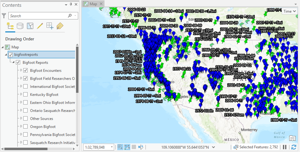
The problem is that Google Earth format files have a limited set of capabilities in ArcGIS Pro so you can’t for example create a selection set or use them in any sort of analysis. They are really only good for visualization purposes. For that reason we are going to need to convert the KMZ file to a feature class in a geodatabase.
If you want to work with the KML features in the same way as other GIS data, use the KML To Layer tool to convert a KML (or KMZ) file to feature classes in a file geodatabase. The tool also creates a corresponding layer file that reflects the symbology established in the KML file.
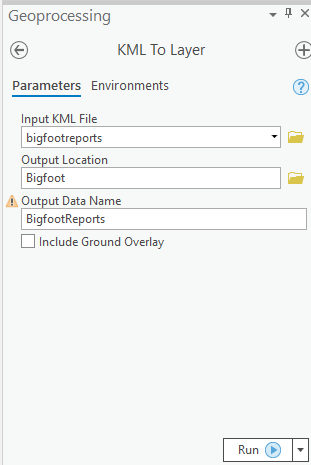
Open the Geoprocessing pane by clicking the Tools button on the Analysis tab in ArcGIS Pro. Find the KML to Layer tool and fill in the parameters as seen in the screenshot below. Note that your output geodatabase should be named Bigfoot if that is what you named your ArcGIS Pro project. You can define whatever name you’d like for the output data name. Run the tool to generate the new feature class.
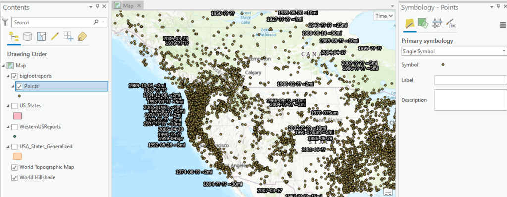
The symbology found in the KMZ file will be ported directly into the output feature class so you may want to use the Appearance tab on the Feature Layer context menu to define a single symbol for the output feature class so that it doesn’t appear so cluttered.
Filtering the Data for Analysis
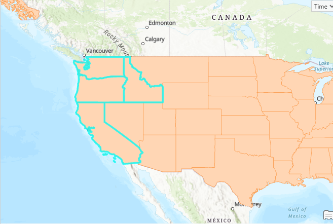
Most analysis project will filter the data by geography or other variables to limit the scope of the project. In this case we’re interested in the spatial analysis of Squatch sightings in the Pacific Northwest. There are a number of definitions of exactly what defines the Pacific Northwest, but for our study we’ll limit it to the states of Washington, Oregon, Idaho, and California.
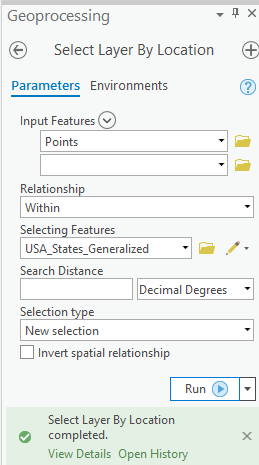
Open the attribute table for the BigfootReports feature class. You’ll notice that it doesn’t have a state indicator so we’re going to need to use the Select By Location tool to filter the sightings that fall within the boundaries of the states in our study area.
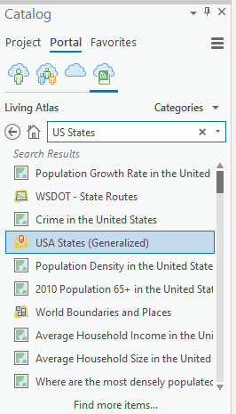
Before running the Select by Location tool you’re going to want to obtain a feature class of US state boundaries. If you don’t have this feature class you can add the USA States (Generalized) feature layer from ArcGIS Online by going to the Catalog pane and clicking the Portal tab and then Living Atlas and searching for US States as seen below. You should be able to drag this layer directly into your map.
Use the Select by Rectangle tool to manually select the states in the study area.
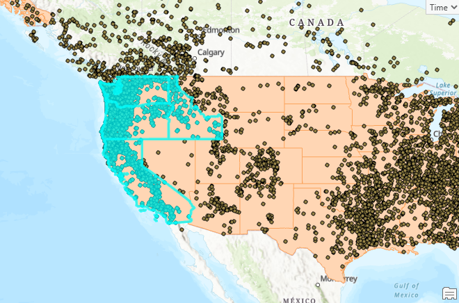
Click the Select by Location tool found on the Map tab. Fill in the parameters as seen below and click Run to select the sightings within the selected state boundaries. You should have 2,272 selected reports.
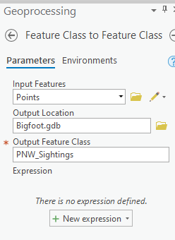
Now we’ll export the selected set of sightings to a new feature class. Right click the Points layer under the bigfootreports group layer and select Data | Export Features. Fill in the parameters as seen below and click the Run button.
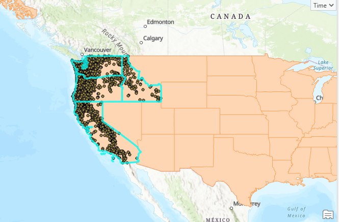
This should leave you with only sightings in the selected states as seen below.
That completes our data preparation stage. Next, we’ll do some basic data exploration.
Data Exploration
For this initial tutorial we’re going to keep the analysis pretty simple and just do a little data exploration before we dive into some deeper analysis tools in future tutorials. We’ll start by aggregating the sightings by county.
Using the skills you learned earlier, find the USA Counties layer by going to Catalog | Portal | Living Atlas and doing a search. Add the layer to your map.
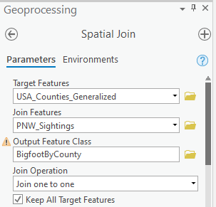
Next we’ll use the Spatial Join tool found on the Feature Layer context menu under the Data tab. This will create a count of the number of sightings per county. The idea behind this step of the process is to aggregate the point data to a larger polygonal area for the purpose of doing various types of spatial analysis. Fill in the parameters as seen below and click the Run button.
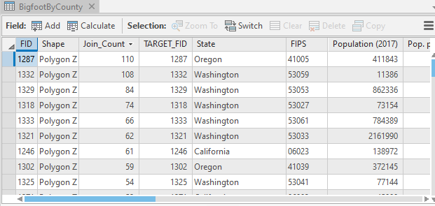
This will generate a new feature class called BigfootByCounty. Open the attribute table for this layer and find the Join_Count field. This contains the number of sightings for each county.
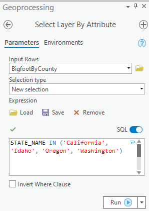
The output still contains every county in the U.S. so use the Select by Attributes tool to select only counties from Oregon, Washington, Idaho, and California. We want to include all counties from those states and not just counties where there have been sightings because we still want to include those counties in future analysis.
Using the skills you learned earlier export the selected counties into a new feature class called BigfootByCountyPNW.
Clean up your table of contents so that only the BigfootByCountyPNW layer is displayed along with your basemap.
Creating a Graduated Color Map
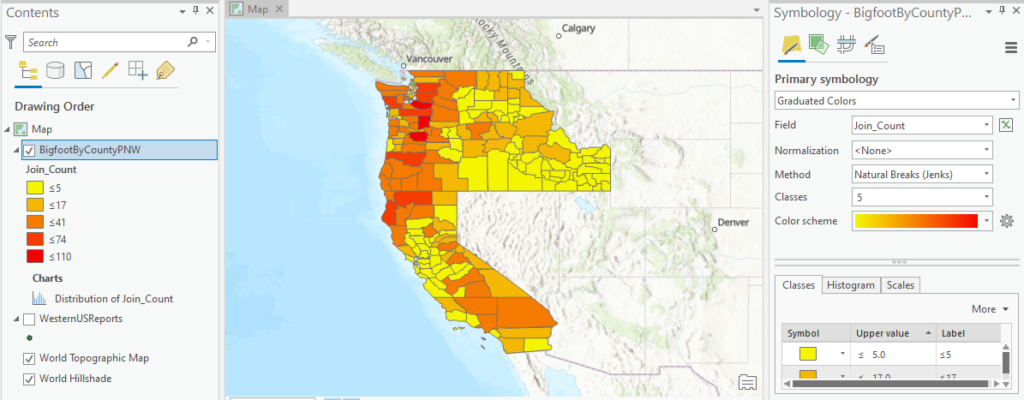
Let’s get a sense of the density of sightings by county by creating a graduated color map. Click the BigfootByCountyPNW layer in the Contents pane. Go to Feature Layer | Appearance | Symbology and selected Graduated Colors. It should automatically create a graduated color map based on some default values including the Join_Count field as seen below.
The big problem with this map is that it doesn’t take the size of the counties into account. Obviously, the more area covered by a county, the more likely it is to have higher counts. We want to take size out of the equation. This is called normalization. Select Shape_Area as the field under the Normalization parameter. You might also select Population or Pop. per Sq. Mi. as other fields to use for normalizing the data.
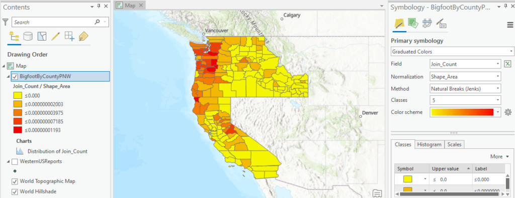
Now we’re starting to see some patterns emerge in our data, with high concentrations of sightings in central and western Oregon and Washington along with northern California and the Sierra Nevada’s. In future tutorial you’ll learn about some additional tools that can be used for hot spot and cluster analysis.
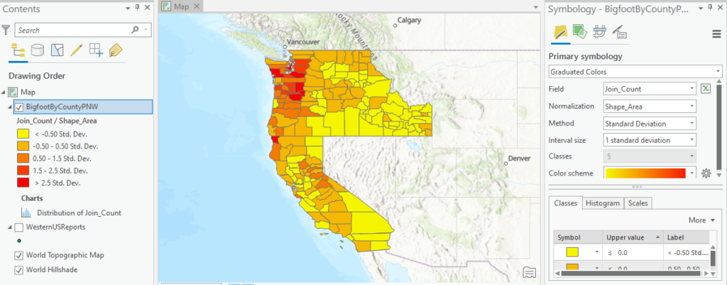
Other parameters that you might want to adjust include the number of classes, method, and color scheme. For example, changing the method to Standard Deviation reveals an even more interesting pattern of density of sightings in Oregon and Washington.
Generating Summary Statistics
It’s also helpful to generate summary statistics about the dataset as well. Open the attribute table for BigfootByCountyPNW and right click the Join_Count field. Select the Statistics option. This will generate a histogram as well as statistics. You should see output as seen in the screenshot below.
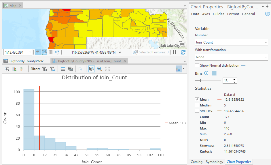
For this dataset we have a mean of 12 sightings per county with a median of 5 and a standard deviation of 18.66.
You can also generate a table of summary statistics for one or more fields by right clicking the Join_Count field and selecting Summarize. This will display the Summary Statistics tool that allows you to select one or more fields, statistics, and case fields.
What’s Next?
In our next tutorial we’ll expand the analysis to include a variety of pattern analysis, clustering, and geographic distribution tools found in the Spatial Statistics toolbox. Later exercises will use R to perform additional analysis of the Sasquatch sightings dataset.
