Prior articles in this series
- Introduction to GIS Analysis using Sasquatch Sightings
- Spatial Squatch – Using the ArcGIS Pro Spatial Statistics Toolbox to Identify Sighting Patterns
- Mapping Clusters of Sasquatch Sightings
In this article I’ll deviate a little from the past three articles in this series that used ArcGIS Pro to perform various types of spatial analysis. In the last article in this series, Mapping Clusters of Sasquatch Sightings, we used the Hot Spot and Optimized Spot Analysis tools in ArcGIS Pro to define hot spots of Sasquatch sightings. We can do something similar with the R programming language with just a few lines of code.
If you are new to the R programming language or programming in general the code you’ll see below may not make much sense to you, but it’s fairly easy to follow and I’ll explain the code as I go. There are lots of good online tutorials that you can use to get up to speed with this highly useful programming language for data analysis including our Introduction to R for Data Visualization and Exploration class.
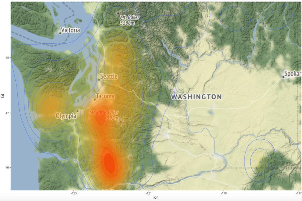
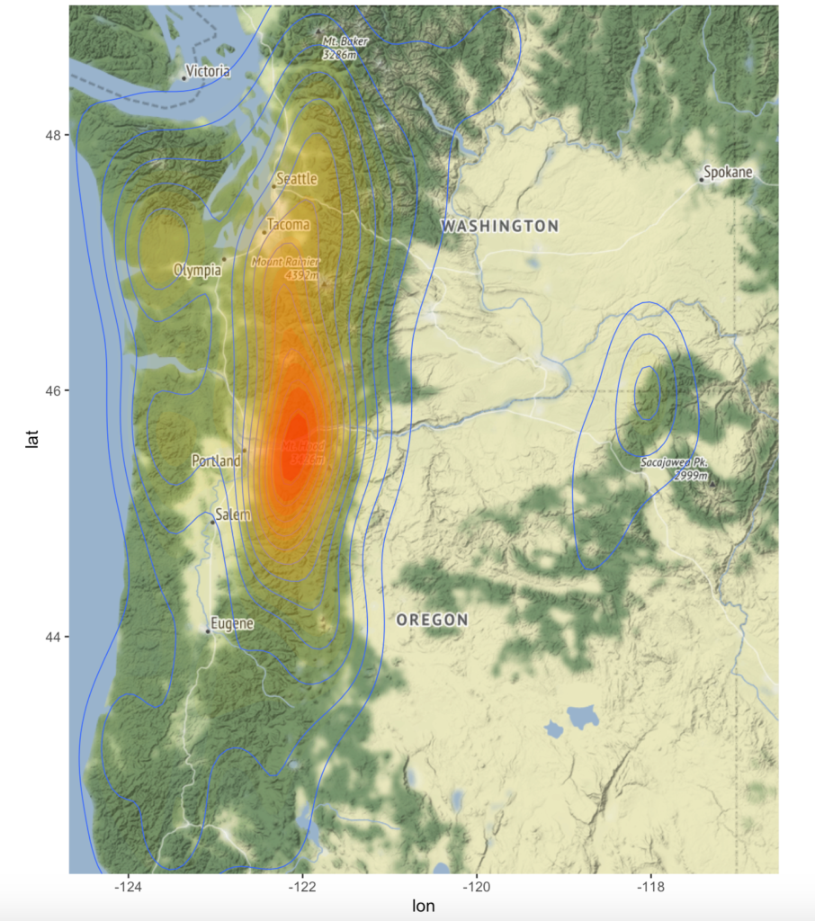
Before we get to the code let’s look at an example of the output from the script we’ll write. I often find that it makes understanding the code easier if you can see an example of what will be produced. Below is a screenshot of a heat map of Sasquatch sightings for the State of Washington. The same point feature class we used in prior articles was used as the input dataset. The heat map displays high concentrations of sightings in red from just south of Tacoma, WA near Mount Rainier south through the Cascade Mountains toward Mount St. Helens. Smaller clusters are found on the Olympic Peninsula and north of Seattle.
Now let’s see how this map was produced with R using the tidyverse, sf, and ggmap packages. You can download the R script and shapefile used to produce this map. We could just as easily used a feature class from a file geodatabase as a shapefile. The sf (simple feature) package in R supports both.
Here is the full script:
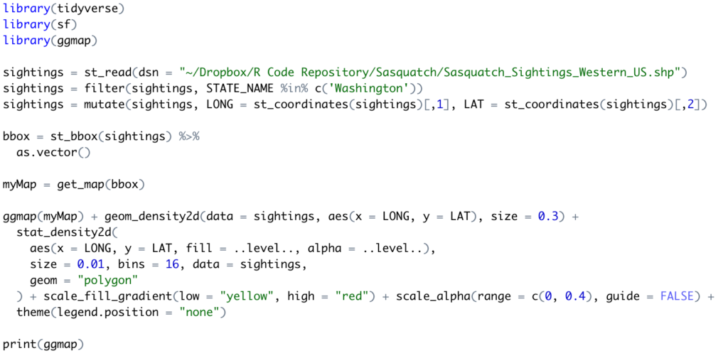
Loading the R Packages
The first few lines of code simply load the R packages that will be used in the script including tidyverse, sf, and ggmap. The tidyverse package is actually a collection of packages for data loading, manipulation, tidying, exploration, and visualization for data science. As an open source programming language, R has thousands of available packages that provide all sorts of functionality. In my opinion though, the collection of packages provided by tidyverse is the pre-eminent set of functionality for data science. In this script we use the dplyr and ggplot2 packages for data manipulation and visualization.
This script also uses the sf package to load the shapefile into an R data frame, which is basically a tabular structure that in this case also includes a column containing the spatial data (points in this case). The ggmap package is also used for basemap creation and the definition of a ggplot2 layer for the Sasquatch sighting data.
Loading and Preparing the Sighting Data
The next few lines of code load the shapefile into a data frame, filter the data to use only sightings from the State of Washington, and add and populate LAT and LONG fields that will be be used later in the script. The st_read() function, found in the sf package, loads the shapefile data (could also have been a feature class from a file geodatabase). I could have also used piping in the lines of code below to simplify the code base, but to simplify the understanding of the code I’ve elected not to do that here.

Creating the Map
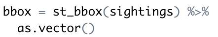
The next couple lines of code use the st_bbox() function from the sf package to get the spatial extent of the data, which will be used later in the creation of the map.
Now it’s time to create the map. These lines of code create a map using the ggmap package defined with the spatial extent of the sighting data. The geom_density2d() and stat_density2d() functions create the contours and heat mapping. Finally, the print() function plots the map.
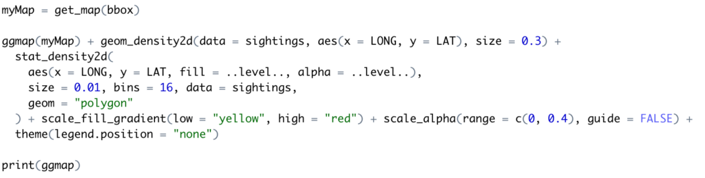
The line of code below can easily be switched out to other states or even combinations of states. Here are a few examples:
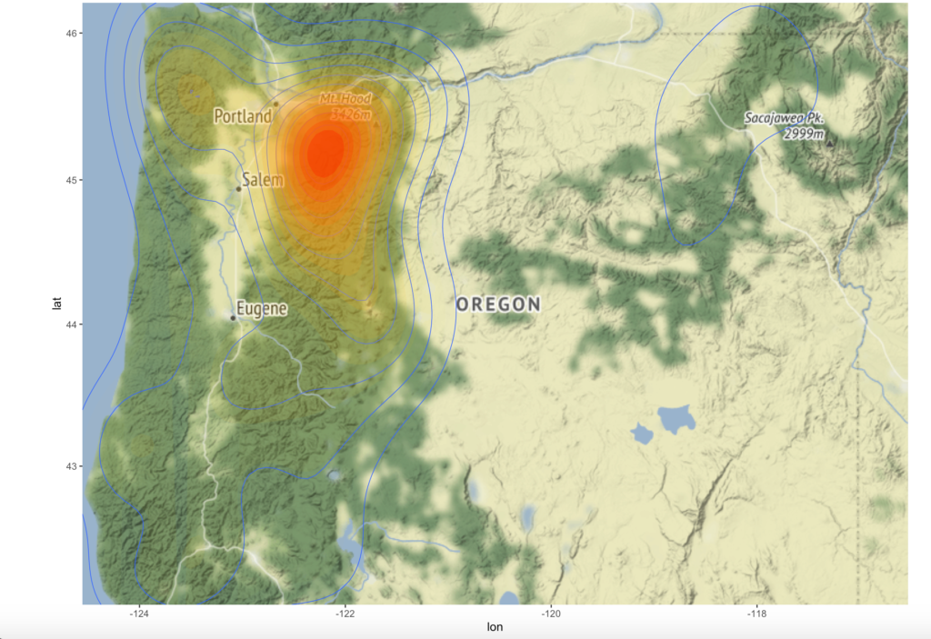
sightings = filter(sightings, STATE_NAME %in% c(‘Oregon’))
sightings = filter(sightings, STATE_NAME %in% c(‘Washington’, ‘Oregon’))
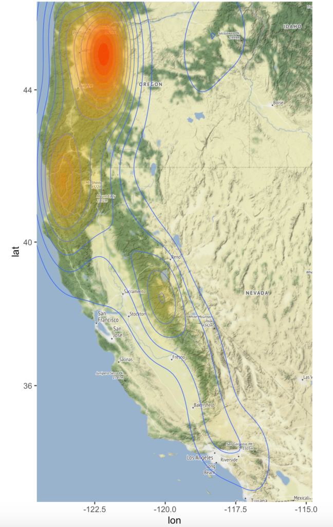
sightings = filter(sightings, STATE_NAME %in% c(‘Washington’, ‘Oregon’, ‘California’))
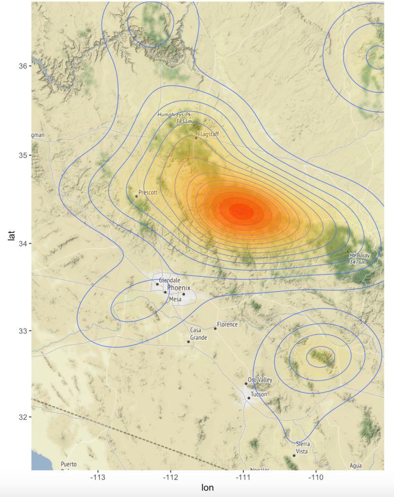
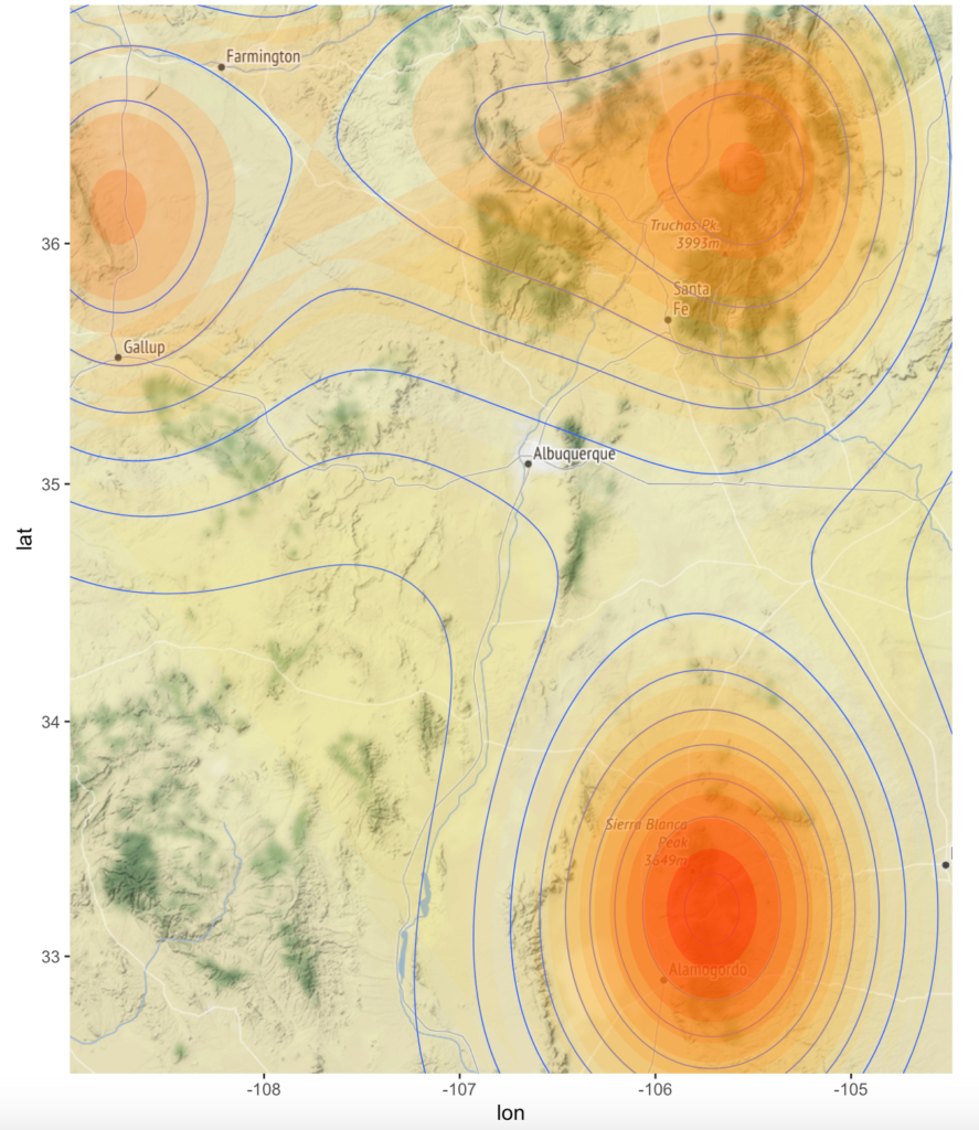
Here are a few of the different heat maps for various states and combinations of states.
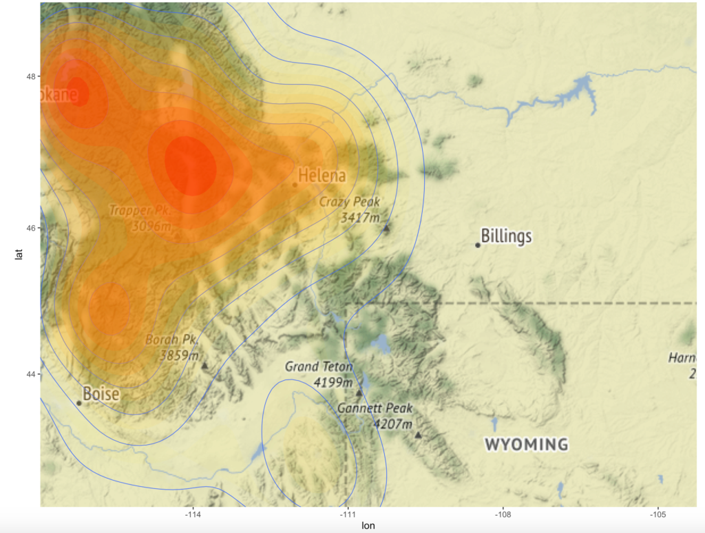
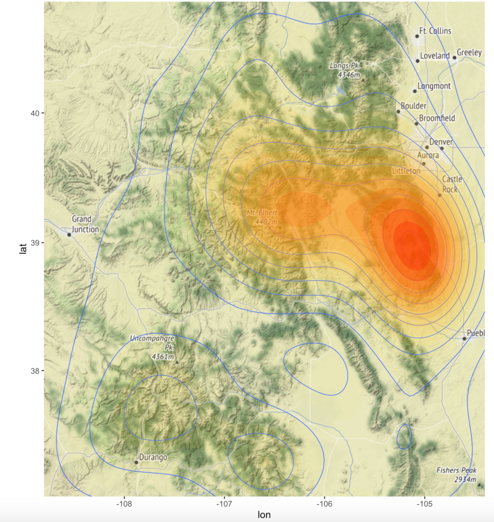
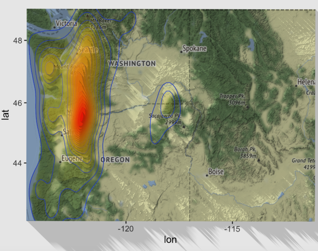
You can also display this data in 3D using the rayshader package as seen below. In the next article in the series we’ll examine the details of how you can use the rayshader package for 3D mapping in R.