Pairwise Buffer vs. Classic Buffer in ArcGIS Pro: What’s the Difference and When Does It Matter?

If you’ve browsed the Geoprocessing toolbox in ArcGIS Pro, you’ve probably noticed a set of tools with “Pairwise” in the name — Pairwise Buffer, Pairwise Clip, Pairwise Intersect, and others. Many users assume these are simply duplicates of the classic tools and never give them a second thought. In reality, the Pairwise tools represent a meaningfully different approach to geoprocessing, with important implications for performance and geometry accuracy.

This article focuses on the most commonly used example — Pairwise Buffer vs. Buffer — to explore what sets the Pairwise tools apart, when those differences matter, and how to choose the right tool for your workflow.

Running a Buffer in ArcGIS Pro: A Quick Walkthrough

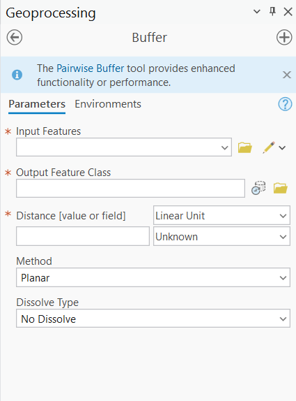
Both the classic Buffer tool and Pairwise Buffer are found in the Analysis Tools toolbox under Proximity. Here’s how to run either one:

1. In the Geoprocessing pane, search for Buffer or Pairwise Buffer and open the tool.
2. Set the Input Features to the layer you want to buffer.
3. Specify the Output Feature Class destination.
4. Set the Distance — either a fixed value or a field-based variable distance.
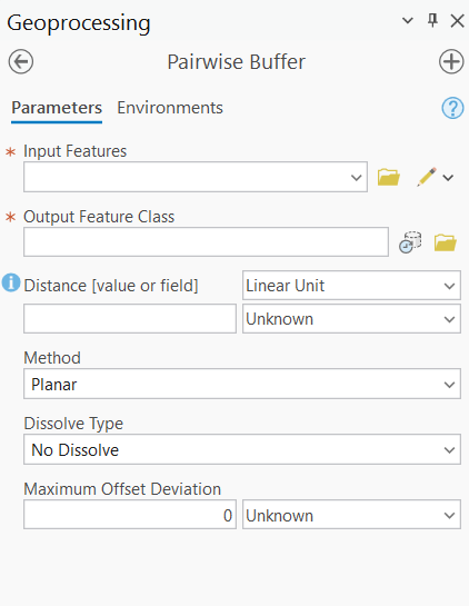
5. Configure optional parameters such as Side Type (Full, Left, Right, Outside Only), End Type (Round or Flat), Dissolve Type, and — in Pairwise Buffer — the Maximum Offset Deviation.
6. Click Run.

At first glance the two tools look nearly identical. The real differences are under the hood — and in one additional parameter that only Pairwise Buffer exposes.

Understanding the Core Differences

1. Parallel Processing and Performance

The most significant practical difference between the two tools is how they use your computer’s processing power.

Classic Buffer was designed in an era of single-core computing. While it can take advantage of parallel processing in some configurations through ArcGIS Pro’s environment settings, it doesn’t do so automatically or consistently. For small datasets, this rarely matters. For large datasets — tens of thousands of parcels, a statewide road network, a national points-of-interest dataset — it can translate into dramatically longer processing times.

Pairwise Buffer was built from the ground up for modern multi-core systems. It uses parallel processing by default, automatically distributing the workload across all available CPU cores without any additional configuration on your part. On a dataset with 500,000 features, the performance difference between the two tools can be substantial — what takes the classic Buffer tool 20 minutes might complete in 4–5 minutes with Pairwise Buffer on the same machine.

The name “Pairwise” actually refers to the underlying processing approach: the tool processes features in pairs or individual chunks across multiple cores simultaneously, rather than working through the dataset sequentially.

2. Geometry Accuracy and the Maximum Offset Deviation Parameter

Buffer zones around points, lines, and polygon edges are mathematically true curves — perfect arcs. However, GIS software doesn’t store true curves in most feature class formats. Instead, it approximates curves using a series of straight line segments, much like a polygon approximating a circle. The more segments used, the smoother and more accurate the curve — but also the more vertices in the output geometry, resulting in larger file sizes and slower downstream processing.

This is where the two tools diverge in an important way.

Classic Buffer handles this approximation internally using a fixed densification approach. You don’t control it directly, and the result is a reasonable approximation that works well for most purposes. However, you have no visibility into or control over the trade-off between geometric accuracy and vertex count.

Pairwise Buffer exposes this control explicitly through the Maximum Offset Deviation parameter. This value defines the maximum allowable distance between the tool’s straight-segment approximation and the true mathematical curve of the buffer boundary. In other words, it sets the tolerance for how closely the output geometry must match a perfect arc.

• Smaller Maximum Offset Deviation values produce more accurate geometry with more vertices — better for precision work, but larger output files and slower downstream analysis.
• Larger Maximum Offset Deviation values produce simpler geometry with fewer vertices — faster processing and smaller files, but a less accurate approximation of the true buffer boundary.

For most workflows, the default value is perfectly adequate. But for applications where geometric precision matters — legal boundary work, infrastructure planning, environmental compliance buffers — having explicit control over this parameter is a genuine advantage.

A Side-by-Side Comparison

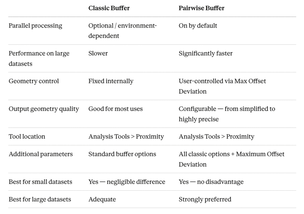
When to Use Each Tool

Use Classic Buffer when:

• Your dataset is small (a few hundred to low thousands of features) and performance is not a concern
• You are following an established workflow or script that already uses the classic tool and there’s no compelling reason to change
• You want the simplest possible tool interface without additional parameters to configure
• You are replicating a legacy analysis where consistency with previous results matters more than optimization

Use Pairwise Buffer when:

• Your dataset is large — tens of thousands of features or more — and processing time matters
• You are running buffers as part of a larger automated workflow or model where cumulative processing time adds up
• You need precise control over the geometric accuracy of the buffer boundary, particularly for regulatory, legal, or engineering applications
• You are working on a machine with multiple CPU cores and want to take full advantage of your hardware (which describes virtually every modern workstation)
• You are building new workflows from scratch — in that case, Pairwise Buffer is simply the better default choice

Our Recommendation

For most ArcGIS Pro users working with typical datasets, Pairwise Buffer is the better default choice — full stop. The parallel processing advantage is real and requires no configuration effort, the geometry control is a genuine added capability, and there is no scenario where Pairwise Buffer produces inferior results to the classic tool. The only reasons to reach for the classic Buffer tool are legacy workflow compatibility or personal familiarity.

If you are building new models, writing new Python scripts using ArcPy, or simply running a one-off buffer analysis, default to Pairwise Buffer. You may not notice the difference on a small dataset, but you’ll be building a habit that pays off significantly when your data gets larger.

A Note on the Other Pairwise Tools

While this article focuses on Buffer, the same logic applies across the entire Pairwise tool family. Pairwise Clip, Pairwise Intersect, Pairwise Dissolve, and Pairwise Erase all share the same core advantage: parallel processing by default with performance benefits that scale with dataset size. If you’re doing heavy overlay analysis on large datasets, swapping classic overlay tools for their Pairwise equivalents is one of the easiest performance wins available in ArcGIS Pro.

Final Thoughts

The Pairwise tools are one of those quiet improvements in ArcGIS Pro that don’t get nearly enough attention. They don’t change what you can do — they change how efficiently and accurately you can do it. Understanding the difference between Pairwise Buffer and the classic Buffer tool won’t just make you a faster analyst; it will help you make more deliberate choices about geometric accuracy and give you better instincts for when performance optimization matters.

Next time you reach for the Buffer tool, take an extra second to consider whether Pairwise Buffer is the better fit. Chances are, it is.