In this tutorial, we’ll be working with graphics layers using raster and vector data. We’ll create an example of a graphic layer to illustrate map features using text and imagery.
What is a graphics layer?
Graphics layers are layers that can contain graphics, such as photos, text as well as geometric shapes, lines and points. These are added on top of map features: they exist as graphics, not as features that contain data records. This means graphic layers are not stored in a geodatabase. Once created, they are part of a Pro project and can be shared with others in multiple ways: as layer files, layer packages and web layers. You cannot create graphic layers larger than 10MB and with more than 4,000 graphic elements. Graphics layers can only be created from 2D maps. Graphic layers can be used to illustrate certain map features with additional information. In this tutorial, we’ll use text and imagery to illustrate a simple map.
How are graphic layers created?
From the “Map” menu on the ribbon interface, click “Add Graphic Layer” to add one to an existing project. You can create multiple Graphics Layers in a single map, and each one can create multiple graphic elements. After a Graphics Layer is created, a new layer is added to the contents pane simply titled “Graphics Layer”. You can change the name of the layer if necessary by double-clicking its name.
Graphics and Graphics Layer menus
Selecting the Graphics Layer in the contents pane highlights two menus on the ribbon interface: a Graphics menu and a Graphic Layer menu. The Graphics menu is used to add graphic elements to the layer: you select an element from the “Insert” box, such as a text box, image or line element. There’s a separate box for styling text elements under “Text Symbol”, while on the left, the Arrange group lets you align, distribute and group multiple graphic elements in a single Graphics Layer. The “Graphics Layer” menu lets you set up a visibility range, and visual effects such as transparency and layer blends. You can also use other map layers as a mask for your graphics layer so they will partly cover your graphics.
STEP 1: Download the data and select the data
We’ll use the Natural Earth quickstart kit. Download and unzip to a file folder location. Open up Pro and create a new map, with a folder connection to the downloaded data. Add the following shapefiles to the map:
- Ne_110m_admin_1_states_provinces.shp
- Ne_110m_populated_places.shp
Make sure the populated places (points) are placed on top of the states and provinces layer so that they are visible in the map window. We’ll now select the state polygon of California. Click the states and provinces layer in the Contents pane and click “Select by Attributes” in the “Map” menu on the ribbon interface. Use the following parameters and click “Run”:
Input Rows: ne_110m_admin_1_states_provinces
Selection Type: New selection
Where “name” is equal “California”
The state boundary of California is highlighted on the map. Right-click the states and boundaries layer in the Contents pane and choose “Selection” and “Make layer from selected features”. Rename the new layer to “California”. We’ll now select the city of San Francisco from the populated places features. Right-click the populated places feature layer and select “Select by Attributes”. Use the following parameters and click OK.
Input rows: ne_110m_populated_places
Selection Type: New selection
Where “NAME” is equal “San Francisco”
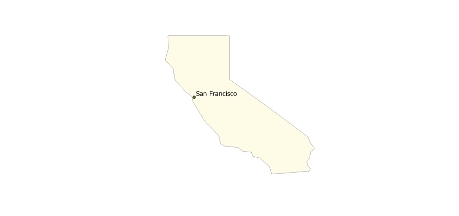
Right-click the populated places layer and choose “Select”, “Make layer from selected features”. Rename the new layer to “San Francisco”. Make sure the two newly created are the only visible layers, so you only have a point feature of San Francisco and a polygon of the state of California. Right-click the San Francisco layer and select “Label” so the city name is added to the map. The results should look like this:
STEP 2: Create the Graphics Layer
Create a new Graphics Layer under “Map” on the ribbon interface, by clicking the button “Add Graphics Layer”. A new layer is added to the Contents pane. First, select the Graphics Layer in the Contents pane and head to the “Graphics Layer” menu to set a reference scale for your map so that you can see the entire map polygon and have sufficient space on the left to add text and images (I used a reference scale of 1:20.719.108).
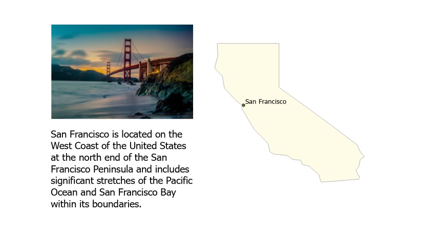
We’ll now add two elements to the new layer: an image of the Golden Gate bridge and some accompanying text from Wikipedia. You can download a free image from the city here and use Wikipedia text for the graphics layer (see the link below). Select the Graphics Layer in the Contents pane and click the Graphics menu. From the Insert menu, choose “Picture” and select an image to add to the map window. You’ll need to make it smaller as it is much larger than the map elements. Next, use the Insert menu to add a Rectangle Text element and add some text about the city (I used the first line from this page). Once you’re done editing both elements, you can decide to group both elements. The results of the new Graphics Layer in the Map window could look something like the image below: