This tutorial shows how to speed up your GIS workflow with three tools that use parallel processing. These tools are recommended for use when you have many features to be processed at once.
GIS analysis often involves the use of buffering, dissolve and clip tools. Using these tools for many features at once may result in slow performance, taking a single operation on many features a long time to finish. Using the following three parallel processing tools, Pro distributes the work to all logical cores on a machine, which results in a much better performance than when using the “normal”, non-pairwise buffer, clip and dissolve tools. We’ll have a look at three examples, using data from the Natural Earth quick start kit.
Step 1: Download the data and open an empty project in Pro
In this tutorial, we’ll be using the ne_10m_admin_0_countries.shp file, which is found in the Natural Earth quick start kit 10m_cultural subfolder. Download the dataset, unzip the files to your hard drive, open a new, empty project and add the shapefile to the map window. Do the same for the ne_10m_admin_1_states_provinces.shp file which is found in the same subfolder.
Step 2: Apply pairwise buffering to the countries file
The countries file contains 255 polygons. Buffering each of them using the normal Buffer tool will take more time than using the Pairwise Buffering tool, that is visible when clicking the “Analysis” tab on the ribbon interface, or clicking “Tools” under analysis and use the search box. This is not necessary for this tool as it is directly visible on the ribbon interface.
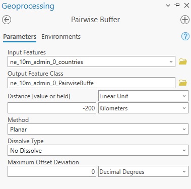
Click the Pairwise Buffering tool and use the parameters listed below. We’ll use a negative value of -200 to create buffers only inside the polygons themselves, instead of both outside and inside. Notice that you can also use a field name with buffer distances for individual features for the Distance field by changing “Linear Unit” to “Field” and selecting the field name of choice. For now, leave the Linear Unit field as it is and select “kilometers” as the field unit. Leave the other settings untouched, run the tool and notice the improved performance in creating the buffers.
Step 3: Apply pairwise clipping
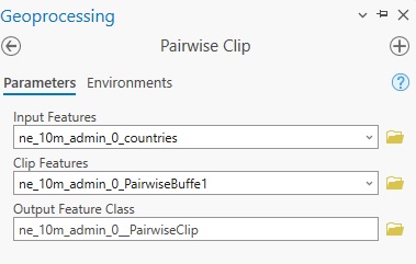
Next, we’ll apply pairwise clipping using the Pairwise Clip tool. We’ll use the newly created buffer polygons (under step 2) as clip features on the larger country polygons. Under Analysis on the ribbon interface, click one of the scroll buttons next to the three displayed analysis tools. Select the “Pairwise Clip” tool and use the following tool parameters and run the tool to see the improved performance here:
You will now only see the inner polygons on the map.
Step 4: Apply pairwise dissolve
Now deselect all feature classes in the Contents pane except the ne_10m_admin_1_states_provinces.shp file. We’ll now use the Pairwise Dissolve tool to dissolve all individual polygons to country files, so that the result will look exactly like the ne_10m_admin_0_countries.shp file. Search for the Pairwise Dissolve tool under “Analysis” on the ribbon interface and run the tool with the following parameters. The country name is listed in the “admin” field, so we need to specify that as the dissolve field:
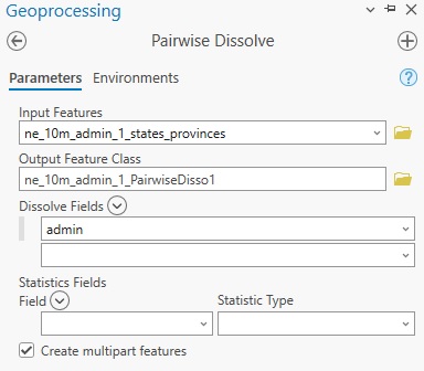
Running the tool with dissolve more than 4,500 features into 253 features in a matter of seconds. Have a look at the results and optionally overlay it with the ne_10m_admin_0_countries.shp file to compare the results: