In a previous article you were introduced to using US Census data using the tidycensus R package. In that article you learned how easy it is to generate R datasets containing either decennial or American Community Survey (ACS) data and visualize that information as plots or maps. In this brief article you’ll learn how to use the simple feature (sf) R package to export this Census data in shapefile format so it can be used in GIS software packages such as ArcGIS or QGIS.
This example will use the get_acs() tidycensus function to extract median monthly housing costs from the ACS for the years 2013-2017 (end year 2017), and 2008-2012 (end year 2012) and generate the percent change between the two time periods. The get_acs() function returns a tidy data frame (called a tibble) that we’ll manipulate to create a final data frame that can then be exported using the sf package. Let’s get to it.
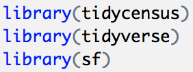
You can access the RPubs markdown file if you want to follow along. As with any other R script you first need to load the libraries that will be used in the script.
To use tidycensus you also need a Census API key, which should be loaded as well.

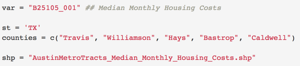
In this next block of code we’re just creating variables to hold the Census variable to extract (B25105 – median monthly housing costs), state and counties, and shapefile name.
Interested in learning more about using R to download, manipulate, explore, and visualize US Census data? Take a look at our new class Exploring and Visualizing Census Data with R.
Next use the get_acs() function to pull ACS data from the end years of 2012 and 2017.

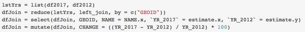
Use the tidyverse reduce() function to join the df2012 and df2017 data frames using the GEOID column. Rename the columns using the select() function, and finally, add a new column called CHANGE using the mutate() function. The CHANGE column will contain the percent change in median monthly housing costs from 2012 to 2017.
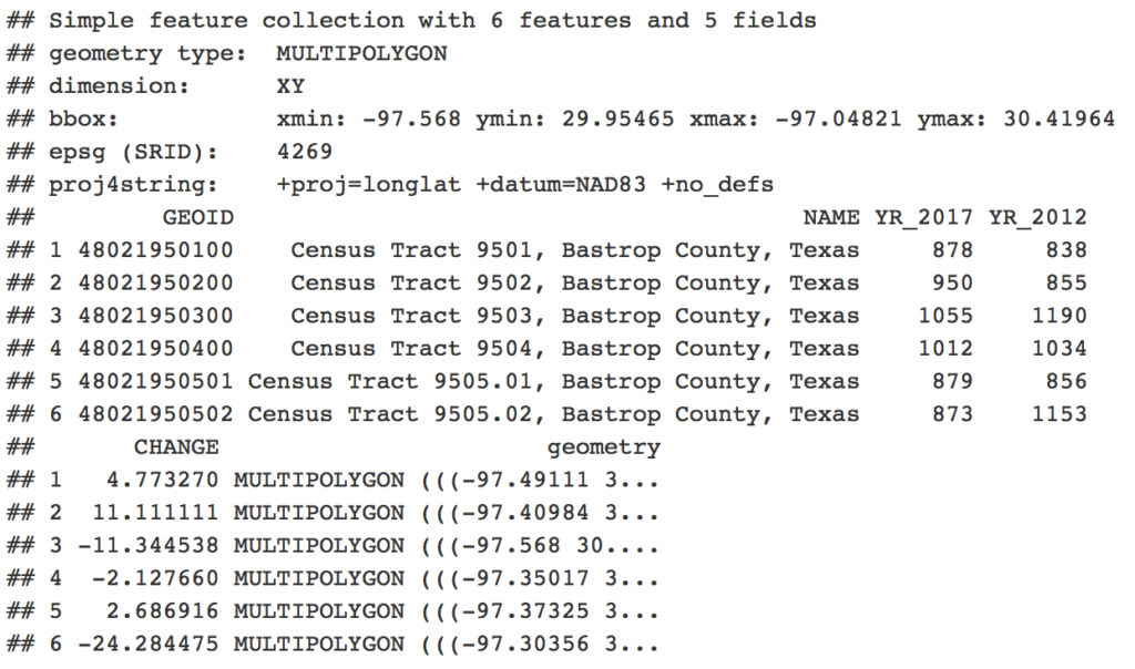
The contents of the dfJoin data frame produced by these last three lines of code can be examined using the head() function. Notice that the data takes the form of a simple feature collection containing the columns GEOID, NAME, YR_2017, YR_2012, CHANGE, and geometry. The geometry column contains the simple feature geometry. All of this information can be written to a shapefile.
head(dfJoin)
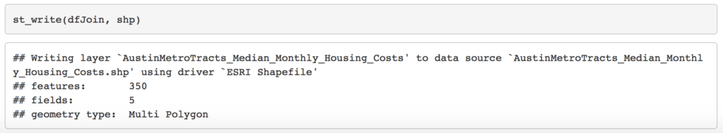
Finally, use the st_write() function from the sf package to write the dfJoin data frame out to a shapefile that can then be used with traditional GIS software.