Analyzing Wildfire Activity with Spatial Analytics – Part 4

Part 1 – Analyzing Wildfire Activity with Spatial Analytics

Part 2 – Analyzing Wildfire Activity with Spatial Analytics

Part 3 – Analyzing Wildfire Activity with Spatial Analytics

In part four of our installment on using spatial analytics to examine wildfire activity in the U.S. we will add a temporal element to the study.  The analysis in this article uses tools found in the Space Time Pattern Mining toolbox in ArcGIS.  They include the Create Space Time Cube, Emerging Hot Spot Analysis, and Visualize Space Time Cube in 2D tools.

Introduction

In GIS, much of our analysis deals with understanding the spatial patterns of our data. However, there are many times when we also need to understand a phenomenon in both space and time. We can expand our idea of things that are closer in space and are more alike to include the idea that things closer in space and time are more related. A space time cube is often used as an input data source to tools in the Space Time Pattern Mining toolbox. In this section we’ll go into more detail on space time cubes, how they are created, and how they are used as input to tools such as Emerging Hot Spot Analysis, and Local Outlier Analysis.

Space Time Cubes

The Create Space Time Cube tool aggregates points into space-time bins. Each bin is basically a cell in 3D. Points from a feature class are aggregated into these space time bins. A count of the number of points in each bin is generated, and the tool can also calculate statistics for attributes if needed. The structure of a space time cube is relatively easy to understand. The X,Y locations define the spatial extent, and the Z defines the time extent. Keep in mind that while a grid type structure like you see below is the default, the tool can also create a hexagonal grid.

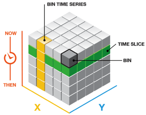
Let’s discuss some of the terminology associated with space time cubes. We’ve already briefly mentioned “bins”. Bins represent a single cell in the space time cube. They represent a specific X,Y spatial extent and time extent. A location, or bin time series, represents a specific X,Y spatial extent through the entire time extent. You can think of a time slice as a layer of information at a specific time interval. For each bin the number of points that fall within the bin are summed.

Space time cubes are used for trend analysis. For example, in our study of wildfire activity, we want to understand if an area is experiencing increasing or decreasing fire activity for a specific area over a period of time.

In order to perform the trend analysis you must have a complete time series. In many cases, bin will have missing values. This can be because there simply weren’t any incidents, or they could indicate another issue. To complete the analysis you need to fill in the empty bins. The Space Time Cube tool provides several ways of filling in the empty bins.

The Create Space Time Cube tool provides several ways of filling in the empty bins. And keep in mind that sometimes you simply don’t have any values for a particular bin. This typically occurs when you’re dealing with incident locations such as crime, fires, traffic accidents, and other similar events. In these cases if there aren’t any events in a bin then it’s perfectly acceptable to fill in the values with zeroes. Another way of filling in empty bins is to use spatial neighbors. This method uses the nearest neighbor values from a specific slice of time to fill in the empty bin. Space-time neighbors uses multiple slices of time, but the same spatial neighbors to fill in the values. And finally, temporal neighbors uses a time series to interpolate the value of a missing bin. This method requires that the first two and last two bins have values for the field.

There are a number of other parameters that can be used when creating a space time cube, but we’ll save discussion of those for later.  For now, let’s move and introduce the Create Space Time Cube tool in ArcGIS.

Using the Create Space Time Cube Tool in ArcGIS

The Create Space Time Cube tool has several required parameters including an input point feature class, and output file name and location for the cube, and a field in the point feature class that represents date/time.  This field must be a Date data type field.  You can see the dialog for the tool in the screenshot below.

In one of the earlier articles in this series we created a point feature class called HistoricalWildfiresPrj.  If you haven’t already created this feature class you’ll want to go back through the first three articles linked at the top of this post.  This feature class contains unique point locations for wildfires that occurred between 2002 and 2015 across the United States.  We’re going to need to perform some additional data manipulation on this feature class before using it in the Create Space Time Cube tool.

• In ArcMap, add the HistoricalWildfiresPrj feature class from the USGS Wildfire Data geodatabase.
• The HistoricalWildfiresPrj feature class contains two fields that contain date information: reportyear and reportdate.  However, both are Text data type fields.  The Create Space Time Cube tool requires a Date data type field so we’ll need to create a new field to hold the date information.  Open the attribute table for the layer and add a new field called STC_Date define it as a Date field.  Use the Field Calculator to populate the STC_Date field with data from the reportdate field.
• The STC_Date field is going to need some cleanup before we can continue with creating the space time cube.  Open the attribute table and sort the STC_Date field in ascending order.  You’ll find quite a few null values, one from the year 800, one from 1999, and one from 2001.  All are outside the time range for the study.  Use the Select by Attribute tool to select all the records where the STC_Date is greater than or equal to 2002-01-01.  This will select 23305 records.
• Export the selection set to a feature class called HistoricalWildfiresTimeCube in the USGS Wildfire Data geodatabase.
• If you zoom to the spatial extent of the HistoricalWildfiresTimeCube feature class you will notice that it includes fires outside the continental U.S.  Let’s clip this feature class to the USCounties_Lower48Prj feature class.  Call the output feature class HistoricalWildfiresTimeCube_Clipped.
• Open the Create Space Time Cube tool and enter the following parameters:
  • Input Features – HistoricalWildfiresTimeCube_Clipped
  • Output Space Time Cube – c:\WildfireData\HistoricalWildfiresTimeCube.nc
  • Time Field – STC_Data
  • Time Step Alignment – END_TIME
  • Distance Interval – 10 Miles
  • Aggregation Shape Type – FISHNET_GRID
• The Create Space Time Cube tool creates a netCDF file.  This space time cube is used as input to other tools found in the Space Time Pattern Mining toolbox such as the Emerging Hot Spot Analysis tool.

Emerging Hot Spot Analysis

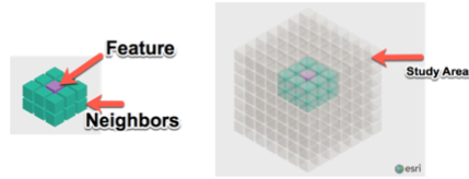
The Emerging Hot Spot Analysis tool identifies clusters in counts to perform a trend analysis. It highlights new, sporadic, oscillating, intensifying, and diminishing hot and cold spots using a space time cube as it’s input.  The Emerging Hot Spot Analysis is calculated very similar to the regular hot spot analysis tool, but with the addition of time as defined in the space time cube.  Ultimately the concept is the same. We compare the neighborhood of a bin to the study area. If it is significantly different than the study area, then the bin is assigned as either a hot or cold spot.

Follow the steps provided below to create an emerging hot spot layer using the space time cube created in the last section of this article.

• In ArcMap find the Emerging Hot Spot Analysis tool in the Space Time Pattern Mining toolbox and open it.
• Enter the following parameters:
  • Input Space Time Cube – C:\WildfireData\HistoricalWildfiresTimeCube.nc\
  • Analysis Variable – Count (this is a count of the number of wildfires that fell within each bin
  • Output Features – C:\WildfireData\USGS Wildfire Data.gdb\HistoricalWildfires_EmergingHotspots
  • Neighborhood Distance = 48205 Meters
  • Neighborhood Time Step – 14
  • Polygon Analysis Mask – USCounties_Lower48Prj
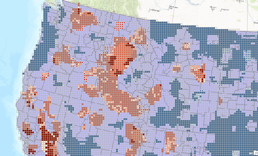
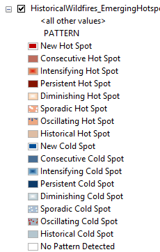
• The tool will create a new feature class that should look similar to the screenshot at the bottom of this post.
• You might be wondering how to interpret the output feature class symbology.  There are certainly a lot of categories that are created with this tool, but keep in mind that the output symbology can be changed.  For example, you might want to group several of the categories together to clarify the output.  Esri provides a help page that can help you interpret the output.  In general it breaks up hot and cold spots into multiple categories including historical, oscillating, sporadic, diminishing, persistent, intensifying, consecutive, and new.  The help page will give you more information on exactly how each feature category is created.

Time-Lapse of Wildfires using Carto and Torque

I also uploaded the HistoricalWildfiresTimeCube layer to Carto.com and applied a Torque styling to the data to produce the time-lapse hot spot map.

Conclusions

Trend analysis enables us to better understand how a phenomenon changes across space and time.  In the case of wildfires we can get a better understanding of areas that have remained persistently hot (or cold), which areas are emerging as new hot spots or that are intensifying, and those that are diminishing or sporadic.

More information on Spatial Analytics:

• Need help with a spatial analytics, data science, or data visualization project?  Get more information on our consulting services.
• Class – Introduction to Spatial Statistics using ArcGIS and R
• Class – Python for Data Science I: Python programming and efficient data management (Pandas)
• Class – R for Data Science I: R Programming and Efficient Data Management
• Book – Spatial Analytics in ArcGIS
• Services – Spatial Statistics and Data Science