In this tutorial, you’ll learn how to use basic pandas functionality to select and manipulate data from a spatially enabled dataframe in a python notebook.
Pandas is a fast, powerful, flexible and easy to use open source data analysis and manipulation tool, built on top of the Python programming language. Because it is included in a default ArcGIS Pro installation, you can use it analyze and manipulate pandas dataframes or spatially enabled dataframes. This tutorial covers some basic pandas functionality to start using pandas.
STEP 1: Download the data
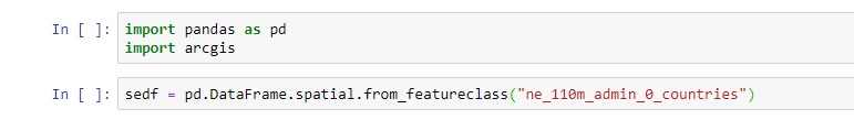
In this tutorial, we’ll be using the ne_110m_admin_0_countries.shp file, which is found in the Natural Earth quick start kit. Download the dataset, unzip the files to your hard drive, open a new, empty project and add the shapefile to the map window. Create a new python notebook in Pro and use the following code snippets to load the pandas and arcgis libraries, as well as creating a spatially enabled dataframe of the shapefile’s attribute table:
The sedf object contains a reference to the attribute table of the shapefile’s row and column data, including a shape field for each row. Because it is based on a pandas dataframe, you can use all available pandas functionality to manipulate and analyze it. The following is only a small sample of what functionality is available.
STEP 2: Investigating the data
There are various ways to have a quick look of a small size of the data. Because the shapefile we’re using here has 117 rows, it’s not a good idea to investigate each row individually. We are better off using a small sample of the data. The following three options all give you a different subset of the data:
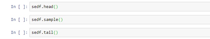
“Head” will give you the first five rows and all columns, “tail” the last five rows, while “sample” will give a you a randomly selected single row back to investigate the data you’re dealing with.
STEP 3: Investigating data types You can get an overview of all data types per column using the following snippet:
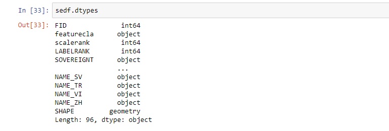
As you can see, it only returns the data types of the first and last five columns. For listing the data types of all columns at once, use “sedf.info()”.
STEP 4: Selecting row and column data
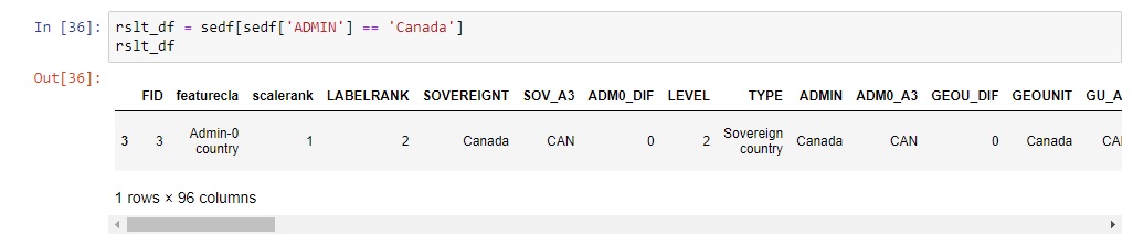
Suppose you want to select a row based on a condition. For example, you only want to see the row(s) where “ADMIN” evaluates to “Canada” (as does the fourth row). To do this, use the following code snippet:
Selecting an entire column is more straight forwarded, as you can use a single command. For example, listing only the “NAME” column would work using “sedf[‘NAME’]”. Unfortunately, pandas only returns the first and last five rows. You’ll have more luck using the “.loc” command. Use this code to select both row and column values for a selection of rows and columns:
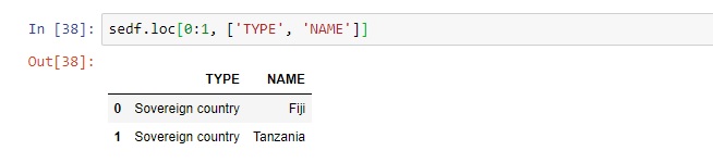
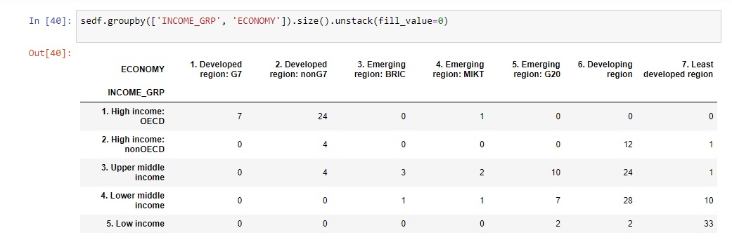
In this example, we’ve selected only two rows and two field values per row. Finally, a very powerful function is the groupby(), which mimics an SQL query. This way, we can group a pandas DataFrame by one or more columns. For example, we can group both the “ECONOMY” and “INCOME_GRP” columns to see if developed regions have higher incomes than lesser developed regions (which seems logical). The query results show that this is indeed the case: